23 min read
Making AI feel realtime with hybrid segmentation
Segmentation is the substrate for nearly every AI photo workflow worth shipping in 2026 — inpainting, object swaps, controlled generation. Here is how to make it feel instant on the web by splitting SAM2 across a notebook on the user's hardware and a decoder in their browser.
On this page
Most "AI on the web" demos punt the hard part to a server: upload an image, spin a loader, pray the queue isn't deep, paint the result. That's fine for a proof of concept and miserable as a product. The real win — the thing that turns a model into a tool people use without thinking — is when the loop closes in under 100 ms and the model feels like a brush, not an API.
This article is about how to get there for interactive segmentation, the
substrate of every modern photo workflow worth shipping: inpainting,
background swap, object replacement, controlled image generation, smart
selection. We'll do it with the best model in its class
(sam2.1_hiera_large, 224M parameters), without compromising on quality, and
without paying a GPU bill per click.
The trick is a deliberately weird deployment: the encoder runs on the user's own machine via a notebook, the decoder runs in their browser tab. Two halves of the same model living on opposite sides of the network, joined by a 16 MB binary blob.
Run / Deploy / Read
Pick the path that matches your hardware and patience
What "segmentation" actually is, and why image generation needs it
Segmentation is the task of assigning a label to every pixel of an image — "this pixel is part of the dog, that one is grass, this one is sky." It's the difference between knowing there's a dog (classification), knowing roughly where the dog is (detection, a bounding box), and knowing the exact silhouette of the dog (segmentation, a mask).

A pixel-level mask is what makes "AI photo editing" actually feel like editing. Source: ClickSEG (Apache 2.0).
That mask is the load-bearing primitive for almost every modern image workflow:
- Inpainting & outpainting: a diffusion model needs to know which pixels to regenerate. The mask is the input.
- Object replacement / removal: lift the masked region out, run a generator on the hole, composite back. Whole product categories (Photoroom, Magic Editor, every "Remove background" feature) are this pipeline.
- Controlled image generation: ControlNet and its descendants take a mask as the spatial prior. "Generate a dragon here" only works if you have a here.
- Annotation pipelines: training data for any pixel-level model (medical imaging, autonomous driving, satellite analysis) is built by humans clicking, refining, and exporting masks. Faster clicks = more data.
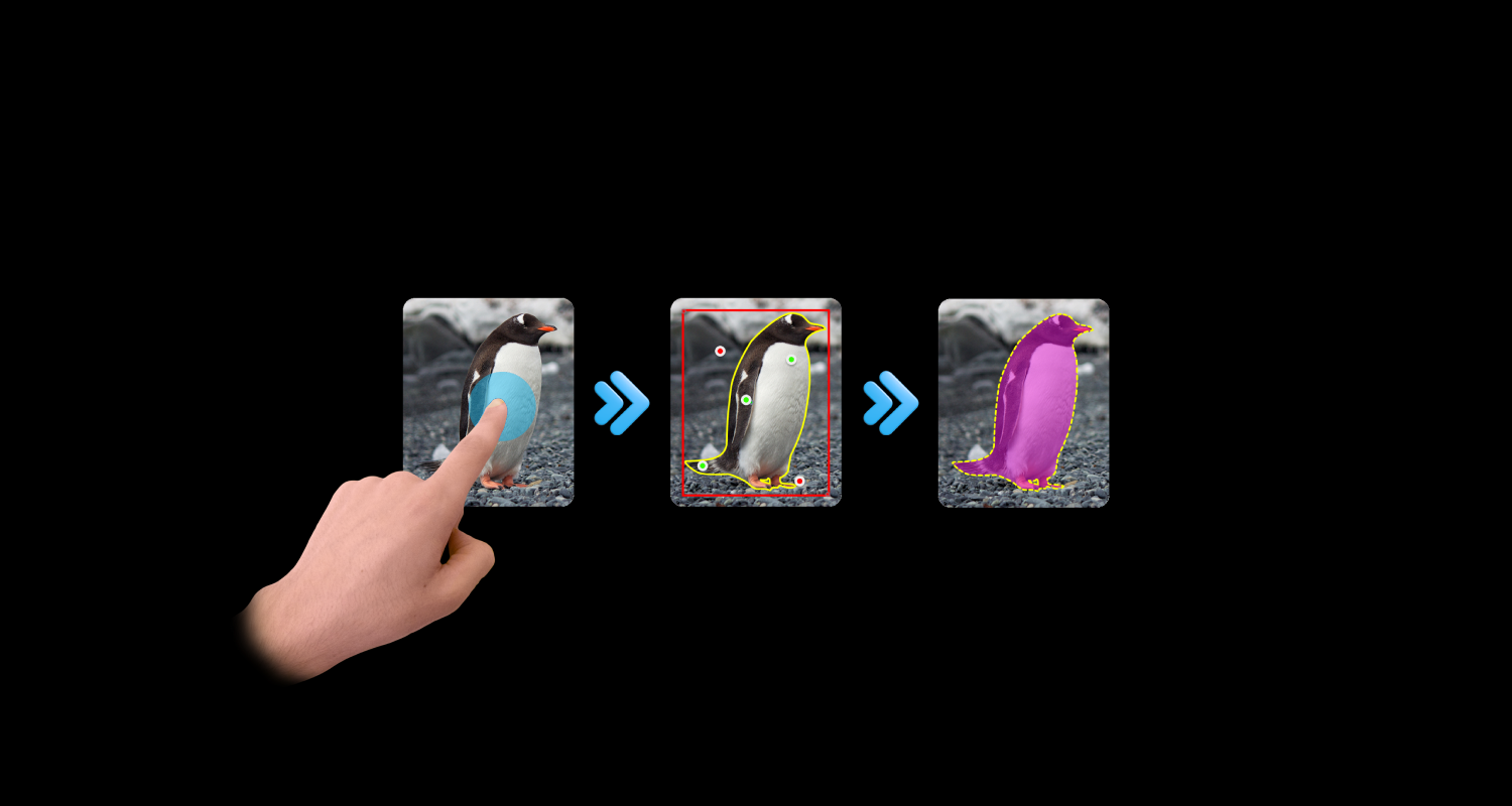
There are two flavors worth distinguishing. Semantic segmentation outputs one mask per category for the whole image — "here's all the road, here's all the sky." Interactive segmentation is the one we want today: the user clicks a point (or drags a box), and the model returns the mask of that specific object, refining as more clicks come in. Add a positive click to grow the selection; add a negative click to fix a region the model got wrong.

Positive (green) clicks recover false negatives; negative (red) clicks cut false positives. SAM2's decoder takes both natively. Source: ClickSEG (Apache 2.0).
The grandparent of the modern interactive segmentation lineage is Meta's SAM (2023), and the child we're using is SAM2, which adds video, better quality on small objects, and a feature pyramid that's friendly to the split deployment we're about to build. The lineage of open interactive segmentation research — CDNet, FocalClick, RITM, SegFormer-based clickers, ClickSEG — is well worth reading if you want to understand the design space; SAM2 is the current top of that tree.
What ONNX is, and why it lets us do this at all
The other half of the story is ONNX: Open Neural Network Exchange. A file format and a runtime ecosystem that lets you take a model trained in PyTorch, serialize its compute graph plus weights to a single artifact, and run it anywhere there's an ONNX runtime — which now means basically everywhere:
| Surface | Runtime | Backend |
|---|---|---|
| Server / Linux x86 | onnxruntime (Py / C++) | CUDA, TensorRT, OpenVINO, CPU |
| macOS | onnxruntime + CoreML EP | Apple Neural Engine, Metal |
| Browser | onnxruntime-web | WebGPU, WASM, WebGL |
| iOS / Android native | onnxruntime-mobile | NNAPI, CoreML, XNNPACK |
| React Native | onnxruntime-react-native | wraps the mobile runtimes |
| Edge / IoT | onnxruntime ARM builds | CPU, NPU |
The point is not that ONNX makes models faster — it doesn't, by
itself. The point is that ONNX decouples the model from the framework,
so the same decoder.onnx file can run via WebGPU in Chrome, via CoreML on
a Mac, via CUDA on a server, and via NNAPI on Android, with no change to the
weights. For a hybrid deployment like the one in this article, that's what
makes the whole shape possible: serialize once, ship the artifact across the
network, let the user's local runtime pick the fastest backend it has.
Try it — right now, in your browser
Before any architecture diagrams — here's the actual decoder running
locally against a pre-encoded portrait. Left-click adds an include point,
right-click adds an exclude point. The View toggle switches between mask
overlay, cutout (transparent background), and erase.
That's sam2.1_hiera_large.decoder.onnx (~16 MB) running in your
tab, fed by an embedding bundle that was produced once on a separate
machine. No server is being hit by your clicks; the only network requests
are the decoder weights and the embedding bundle, both fetched once at page
load. Every click after that is local inference.
Stop reading and play with it for a moment. Notice the latency. That's the entire point.
The architecture
SAM2 is unusually friendly to this kind of split, and that's not an accident — Meta designed the original SAM with interactive use in mind, and SAM2 inherited the same two-stage shape. Conceptually:
The encoder is a heavy Hiera vision transformer that produces a fixed-size feature pyramid for the whole image. The decoder is a small transformer that takes those features plus a prompt and produces a mask. Crucially, the encoder's output does not depend on the prompt. Once an image is encoded, the decoder can run thousands of times with different clicks and never touch the encoder again. That's the entire asymmetry the architecture exploits:
| Operation | Cost (sam2.1 large) | Frequency |
|---|---|---|
| Encode image | 8–10s on Apple Silicon GPU | Once per image |
| Decode w/ prompt | 30–60ms on WebGPU | Once per click/drag |
| Embedding size | ~16 MB float16 (compressed) | Transferred once |
For consumer products, hybrid deployments — encoder on a backend, decoder client-side — are the production-grade pattern that companies like Labelbox have settled on. For a developer-facing demo, a research tool, or anything where the audience is technical, we can go one step further:
Let the user run the encoder. The image never leaves their machine, the GPU bill is theirs (or zero if they use Colab), and we get to ship the large model on both sides without a 360 MB browser download.
Step 1 — Export the models
Pretrained SAM2 checkpoints are PyTorch. We need ONNX, and we need the
encoder/decoder pre-split — you don't get this from a naïve
torch.onnx.export because the official model is a single Predictor that
wraps both stages. The samexporter package handles the surgery.
Run / Deploy / Read
Pick the path that matches your hardware and patience
The notebook is a single file with five cells. Pick a tab to read each one; they run in order top-to-bottom and are all you need to get from a JPEG to the deployable embedding bundle:
# Cell 1 — pin a working torch + the ONNX toolchain.
pip install --quiet \
  torch==2.4.0 \
  torchvision==0.19.0 \
  onnx onnxscript onnxsim onnxruntime samexporter

pip install --quiet git+https://github.com/facebookresearch/segment-anything-2.gitA few things worth knowing about this step that the official docs gloss over:
- The 2 GB ONNX size limit kicks in here. The encoder exceeds it,
so the exporter automatically produces an
.onnxfile plus an external.onnx.datafile containing the weights. Both must live in the same directory at load time. Combined size lands around 850 MB — manageable on disk, untenable as a browser download. This is one of the reasons we keep the encoder off the client. samexporteris doing real work, not just a re-export. It splits the graph at the right boundary, sets up dynamic axes for variable point counts in the decoder, and configuresmultimask_output=Trueso the decoder returns three candidate masks plus IoU predictions per call.- The decoder is tiny. ~16 MB after export, slots comfortably into a Vercel deployment's static assets. Vercel's CDN gzips it on the way down to ~12 MB.
Step 2 — Encoding details, in plain English
The encoder takes a fixed 1024×1024 RGB tensor (normalized with ImageNet
statistics) and returns three outputs — the SAM2 feature pyramid:
image_embed: shape(1, 256, 64, 64)— the main embedding.high_res_feats_0: shape(1, 32, 256, 256)— high-resolution features for the decoder.high_res_feats_1: shape(1, 64, 128, 128)— another resolution level.
If you've worked with SAM1 before, this catches you off guard — SAM1 ships a single embedding tensor; SAM2 plumbs three. All three are needed by the decoder.
The naïve packaging is to save them as float32, which gives you a ~50 MB file per image. We do better with two tricks: cast to float16 (SAM2's decoder is robust to it; size halves), and use a flat binary layout with a JSON manifest beside it (avoids a numpy reader in the browser). Combined, the bundle lands at ~12–18 MB depending on the image's high-frequency content.
Step 3 — ONNX details that shape the JS code
The decoder's interface is the contract you'll be coding against in the browser. Inputs:
| Name | Shape | Notes |
|---|---|---|
image_embed | (1, 256, 64, 64) | from the encoder |
high_res_feats_0 | (1, 32, 256, 256) | from the encoder |
high_res_feats_1 | (1, 64, 128, 128) | from the encoder |
point_coords | (1, N, 2) | in 1024×1024 model space |
point_labels | (1, N) | 1=fg, 0=bg, -1=padding |
mask_input | (1, 1, 256, 256) | previous mask, or zeros |
has_mask_input | (1,) | 0.0 ignore, 1.0 use |
Outputs: masks (1, 3, 256, 256) float32 logits (threshold at 0,
upsample), and iou_predictions (1, 3) float32 (pick the top one).
Resolution upgrade we ship in the template. The default samexporter export emits 256×256 mask logits — fine for line work but visibly stair-stepped on a phone-camera selfie at 1500+ display px. The repo ships
scripts/export_decoder_hires.py, a one-file subclass that adds an in-graphF.interpolate(size=512)on the mask output. Same weights, same encoder bundle (image_embed/high_res_feats_*are unchanged), butdecoder.onnxnow returns(1, 3, 512, 512). Halving the upscale factor to display kills the source-grid checker that SAM2's clamped logits would otherwise produce in textured regions.
Coordinate space. Points must be in the 1024×1024 model input space, not the original image's space and not the canvas's pixel space. This catches everyone the first time:
const x = (cx / canvasWidth)  * 1024;
const y = (cy / canvasHeight) * 1024;
Encoder vs decoder optimization. For the encoder we'd convert the
.onnx to ONNX Runtime's .ort format with
python -m onnxruntime.tools.convert_onnx_models_to_ort for faster load.
For the decoder this conversion sometimes fails on a Concat node
— the plain .onnx works in the browser, so we leave it alone.
Community-known quirk that the official docs don't really mention.
Step 4 — The Vercel app
The web app is a Next.js project deployed to Vercel. Structure:
/app/page.tsx                # main UI: image picker + canvas
/components/Segmenter.tsx    # canvas + click handling
/lib/sam2-decoder.ts         # ONNX session + inference
/public/models/decoder.onnx  # ~16 MB, ships with the deploy
/public/demos/<slug>/        # preview.jpg + embedding.bin + manifest.json
/public/workers/sam2-decoder-worker.js
A note on Vercel limits: 100 MB hard cap on serverless function bundles; static assets are looser. The 16 MB decoder is fine. Each demo embedding is ~16 MB; you can ship 3–5 of these comfortably. For more, push to R2/S3 and serve via CDN.
Run / Deploy / Read
Pick the path that matches your hardware and patience
The Deploy-to-Vercel button clones the template repo, prompts you for two
optional env vars (REPLICATE_API_TOKEN and NEXT_PUBLIC_REPLICATE_MODEL),
and you get a working deployment with the demo embeddings baked in. If you
skip the Replicate vars, the app still works for pre-baked demos and
notebook-uploaded files.
Loading the decoder on WebGPU
In the browser we use onnxruntime-web with the WebGPU execution provider.
The whole decoder lifecycle is small enough to fit in one file:
import * as ort from "onnxruntime-web/webgpu";

export interface Embedding {
  imageEmbed: ort.Tensor;
  highResFeats0: ort.Tensor;
  highResFeats1: ort.Tensor;
  originalWidth: number;
  originalHeight: number;
}

export async function loadDecoder(): Promise<ort.InferenceSession> {
  return ort.InferenceSession.create("/models/decoder.onnx", {
    executionProviders: ["webgpu"],
    graphOptimizationLevel: "all",
  });
}

export async function loadEmbedding(slug: string): Promise<Embedding> {
  const [manifest, buffer] = await Promise.all([
    fetch(`/demos/${slug}/manifest.json`).then((r) => r.json()),
    fetch(`/demos/${slug}/embedding.bin`).then((r) => r.arrayBuffer()),
  ]);

  const toTensor = (name: string) => {
    const t = manifest.tensors[name];
    const f16 = new Uint16Array(buffer, t.offset, prod(t.shape));
    // ORT-web doesn't accept fp16 ArrayBuffers directly for all ops;
    // expand to fp32 once on load (~50ms for a large embedding).
    const f32 = new Float32Array(f16.length);
    for (let i = 0; i < f16.length; i++) f32[i] = f16ToF32(f16[i]);
    return new ort.Tensor("float32", f32, t.shape);
  };

  return {
    imageEmbed:    toTensor("image_embed"),
    highResFeats0: toTensor("high_res_feats_0"),
    highResFeats1: toTensor("high_res_feats_1"),
    originalWidth: manifest.originalWidth,
    originalHeight: manifest.originalHeight,
  };
}

export async function segment(
  session: ort.InferenceSession,
  emb: Embedding,
  clicks: { x: number; y: number; positive: boolean }[],
  canvasWidth: number,
  canvasHeight: number,
): Promise<Float32Array> {
  const coords = new Float32Array(clicks.length * 2);
  const labels = new Float32Array(clicks.length);
  clicks.forEach((c, i) => {
    coords[i * 2]     = (c.x / canvasWidth)  * 1024;
    coords[i * 2 + 1] = (c.y / canvasHeight) * 1024;
    labels[i]         = c.positive ? 1 : 0;
  });

  const out = await session.run({
    image_embed:      emb.imageEmbed,
    high_res_feats_0: emb.highResFeats0,
    high_res_feats_1: emb.highResFeats1,
    point_coords:     new ort.Tensor("float32", coords, [1, clicks.length, 2]),
    point_labels:     new ort.Tensor("float32", labels, [1, clicks.length]),
    mask_input:       new ort.Tensor("float32", new Float32Array(256 * 256), [1, 1, 256, 256]),
    has_mask_input:   new ort.Tensor("float32", new Float32Array([0]), [1]),
  });

  const masks = out.masks.data as Float32Array;            // (1, 3, 256, 256)
  const iou   = out.iou_predictions.data as Float32Array;  // (1, 3)
  let best = 0;
  for (let i = 1; i < 3; i++) if (iou[i] > iou[best]) best = i;
  return masks.slice(best * 256 * 256, (best + 1) * 256 * 256);
}

const prod = (arr: number[]) => arr.reduce((a, b) => a * b, 1);

function f16ToF32(h: number): number {
  const s = (h & 0x8000) >> 15;
  const e = (h & 0x7c00) >> 10;
  const f = h & 0x03ff;
  if (e === 0) return (s ? -1 : 1) * Math.pow(2, -14) * (f / 1024);
  if (e === 0x1f) return f ? NaN : (s ? -Infinity : Infinity);
  return (s ? -1 : 1) * Math.pow(2, e - 15) * (1 + f / 1024);
}
Three operational notes:
- Run the decoder in a Web Worker. A 60 ms forward pass on the main thread eats your animation budget. The previous post covers that pattern.
- Throttle drag interactions with
requestAnimationFrame. Calling on everymousemovequeues dozens of inference jobs and stutters. - Upsample the mask via
<canvas>drawImage. The browser's bilinear resize is good enough and free.
Step 5 — The interactivity loop
The promise the architecture makes is that the click-to-mask loop is instantaneous. Here's what happens, end-to-end:
Click → mask loop
Cold load
Fetch decoder.onnx + first embedding
There's no spinner, no loading state, no API roundtrip. The latency of "round-trip to a server, run inference, send back a PNG" — what most cloud SAM deployments give you — is replaced with sub-100 ms local inference. That is what makes it feel like a tool instead of a demo.
Picking the right execution provider
onnxruntime-web ships several backends, and the choice matters:
| Provider | Cost on the large decoder | Where it works |
|---|---|---|
| WebGPU | 30–60 ms | Chrome, Edge, Safari TP, modern Firefox |
| WASM | 200–400 ms | Everywhere; SIMD makes it tolerable |
| WebGL | (deprecated for this use) | Skip |
The pragmatic pattern is WebGPU first, WASM fallback:
async function createSession(modelUrl: string) {
  try {
    return await ort.InferenceSession.create(modelUrl, {
      executionProviders: ["webgpu"],
    });
  } catch (e) {
    console.warn("WebGPU unavailable, falling back to WASM:", e);
    return await ort.InferenceSession.create(modelUrl, {
      executionProviders: ["wasm"],
    });
  }
}
For the article's demo I'd gate the experience behind a "WebGPU recommended" banner if it falls back. The decoder is small enough to run on CPU, but drag interactions feel laggy and it's worth telling the user why.
Step 6 — Replicate as an alternative to the notebook
Some users won't run a notebook, period. For them, the encoder needs to live behind an API call. The cleanest pattern is bring-your-own Replicate token: we ship a tiny encoder model on Replicate that takes an image and returns the bundle, the user pastes their own API token in the web app, and the upload-image flow becomes one HTTP call instead of "open Colab."
Three reasons this is the right pattern:
- Cost stays with the user. No GPU bill on our side. Replicate charges the user's account directly.
- Privacy is honest. Their image goes to Replicate, not to us. Our server never sees the bytes.
- Trivial to swap. Same
embedding.bin+manifest.jsonshape as the notebook produces. The decoder code in the browser doesn't change.
Run / Deploy / Read
Pick the path that matches your hardware and patience
cog is Replicate's tool for packaging a model. Here's the whole encoder
service — four files, one push command:
build:
gpu: true
cuda: "12.1"
python_version: "3.11"
python_packages:
  - "torch==2.4.0"
  - "torchvision==0.19.0"
  - "onnxruntime-gpu==1.20.0"
  - "Pillow==10.4.0"
  - "numpy==1.26.4"
predict: "predict.py:Predictor"For a Hugging Face Space alternative, the same predict() function ships
inside a Gradio app exposing /api/predict, and huggingface.js hits it
the same way. Pick whichever your audience already has accounts with.
Where this goes from here
The split-inference pattern generalizes well beyond SAM2. Any model with an expensive encoder and a cheap promptable head fits this shape:
- CLIP-style retrieval. Encode a corpus offline, ship embeddings, do nearest-neighbor in the browser. Same pattern.
- Depth-anything / monocular depth. Encode once on a server, refine client-side.
- SAM3 (when it lands). Three-model pipeline (image + language + decoder) is a natural extension — text encoder and image encoder server-side, decoder in the browser.
The notebook-as-encoder pattern is particularly nice for research and developer tools, where the audience is comfortable running Python and the privacy/cost benefits matter. For consumer products, Replicate or a HF Space is the friction-free swap. The browser side stays identical.
The point — worth stating explicitly because it's easy to miss — is that interactive ML on the web doesn't have to mean small, fast, low-quality models. You can ship the best model in its category by being thoughtful about which parts run where. The encoder is heavy and runs once. The decoder is light and runs constantly. Put each one in the place where its cost profile makes sense, and the user gets an experience that wasn't possible five years ago: a 224M-parameter vision transformer responding to their clicks in real time, in a browser tab, with their image never leaving their machine.
Appendix — file checklist
What ships where:
| File | Where it lives | Size |
|---|---|---|
sam2.1_hiera_large.encoder.onnx | User's machine (notebook only) | ~850 MB |
sam2.1_hiera_large.encoder.onnx.data | User's machine (notebook only) | varies |
sam2.1_hiera_large.decoder.onnx | Vercel /public/models/ | ~16 MB |
embedding.bin (per image) | Vercel /public/demos/<slug>/ or uploaded | ~12–18 MB |
manifest.json (per image) | Vercel /public/demos/<slug>/ or uploaded | <1 KB |
preview.jpg (per image) | Vercel /public/demos/<slug>/ or uploaded | varies |
Appendix — sources, reading, distribution
Run / Deploy / Read
Pick the path that matches your hardware and patience
Models & code referenced:
sam2.1_hiera_largecheckpoint — Meta's official Hiera-Large weights.samexporter— the ONNX export tool that handles the encoder/decoder split.onnxruntime-web— the in-browser runtime, with WASM and WebGPU backends.onnxruntime-react-native— same model on phones, via Expo's prebuild plugin.- Pre-exported community models — if you want to skip the export step entirely.
- Cog (Replicate's packaging tool).
- Hugging Face Spaces docs.
Background reading on interactive segmentation:
- Segment Anything (SAM, 2023).
- SAM2: Segment Anything in Images and Videos (2024).
- ClickSEG codebase — CDNet / FocalClick / efficient baselines, the lineage that informed SAM's click-driven interface.
- The earlier post on this site about ONNX in the browser.
Distribution checklist. The share buttons above pre-fill the title and canonical URL for LinkedIn and X. For Medium, publish the canonical version here and use Medium's "Import a story" flow with this URL — it preserves the canonical link tag for SEO. For the LinkedIn long-form post, paste the body and link back to this page; LinkedIn's algorithm tolerates plain text plus one strong outbound link. The "Read with an LLM" buttons at the top of this article point at the raw markdown source — drop that URL into ChatGPT or Claude and it has the whole article in one shot.
Comments
Tags in this post
Keep reading
Running ONNX models in the browser without losing your weekend
A working recipe for shipping image segmentation in a tab — Web Workers, WASM, pre-encoded embeddings, and the small things that decide whether the demo is fast or felt-fast.
4 min · May 4, 2026
Welcome to the new blog
A short tour of the new MDX-powered writing setup, complete with syntax-highlighted code blocks rendered by Shiki at build time.
1 min · May 4, 2026
Rendering Brilliance
A visual tour of the cubemap-based diamond shader — how a faceted gemstone becomes a single texture lookup, and what that gets you. Eight interactive figures, plain-English asides, and the optics that hold it all together.
15 min · May 26, 2026
All tags